3. Surrogate model

3.1. Generalities

A common class is used to manage surrogate models. Hence, several kind of surrogate model strategies can be used:

predictor = batman.surrogate.SurrogateModel('kriging', corners, labels)
predictor.fit(space, target_space)
predictor.save('.')
points = [(12.5, 56.8), (2.2, 5.3)]
predictions = predictor(points)

3.2. From Kriging to Gaussian Process

3.2.1. Kriging, a geostatistical method

Kriging is a geostatistical interpolation method that use not only the distance between the neighbouring points but also the relationships among these points, the autocorrelation. The method has been created by D.G. Krige [Krige1989] and has been formalized by G. Matheron [Matheron1963].

In order to predict an unmeasured location \(\hat{Y}\), interpolation methods use the surrounding measured values \(Y_i\) and weight them:

\[\hat{Y} = \sum_{i = 1}^{N} \lambda_i Y_i.\]

The advantage of this method is that the interpolation is exact at the sampled points and that it gives an estimation of the prediction error. Ordinary Kriging consists in the Best Linear Unbiased Predictor (BLUP) [Robinson1991]:

Best

It minimizes the variance of the predicted error \(Var(\hat{Y} - Y)\),

Linear

A linear combination of the data,

Unbiased

It minimizes the mean square error \(E[\hat{Y} - Y]^2\) thus \(\sum_{i=1}^{N} \lambda_i(x)=1\),

Predictor

It is an estimator of random effects.

\(\lambda_i\) are calculated using the spatial autocorrelation of the data, it is a variography analysis. Plots can be constructed using semivariance, covariance or correlation. An empirical variogram plot allows to see the values that should be alike because they are close to each other cite{Bohling2005}. The empirical semivariogram is given by:

\[\gamma(h) = \frac{1}{2}\times \frac{1}{n} \sum_{i=1}^{N} (Y_i - Y_{i+h})^2.\]

A fitting model is then applied to this semivariogram. Hence, the variability of the model is inferior to data’s. Kriging smooths the gradients. The exponential model is written as:

\[\gamma(h) = C(0) + C\left(1- \exp{\left(-\frac{h}{r}\right)}\right),\]

with \(C\) the correlation matrice and the parameter \(r\) is optimized using the sample points.

A model is described using:

Sill

It corresponds to the maximum of \(\gamma\). It defines the end of the range.

Range

It is the zone of correlation. If the distance is superior to the range, there is no correlation, whereas if the distance is inferior to it, the sample locations are autocorrelated.

Nugget

If the distance between the points is null, \(\gamma\) should be null. However, measurement errors are inherent and cause a nugget effect. It is the y-intercept of the model.

Once the model is computed, the weights are determined to use the MSE condition and gives:

\[\lambda_i = K^{-1}k,\]

\(K\) being the covariance matrix \(K_{i,j} = C(Y_i-Y_j)\) and \(k\) being the covariance vector \(k_i = C(Y_i-Y)\) with the covariance \(C(h) = C(0) - \gamma(h) = Sill-\gamma(h)\).

\[\begin{split}\begin{pmatrix}\gamma_{11}& \cdots & \gamma_{1j} \\ \vdots & \ddots & \vdots \\ \gamma_{i1} & \cdots & \gamma_{nn} \end{pmatrix} \begin{pmatrix}\lambda_1 \\ \vdots \\ \lambda_n \end{pmatrix} = \begin{pmatrix} \gamma_{1X} \\ \vdots \\ \gamma_{nX}\end{pmatrix}.\end{split}\]

Furthermore we can express the field \(Y\) as \(\hat{Y} = R(S) + m(S)\) which is the residual and the trend components [Bohling2005]. Depending on the treatment of the trend, there are several Kriging techniques (ordinary Kriging being the most used):

Simple

The variable is stationary, the mean is known,

Ordinary

The variable is stationary, the mean is unknown,

Universal

The variable is non-stationary, there is a tendency.

Ordinary Kriging is the most used method. In this case, the covariance matrix is augmented:

\[\begin{split}\begin{pmatrix}\gamma_{11}& \cdots & \gamma_{1j} & 1\\ \vdots & \ddots & \vdots & \vdots \\ \gamma_{i1} & \cdots & \gamma_{nn} & 1 \\ 1 & \cdots & 1 & 0 \end{pmatrix} \begin{pmatrix}\lambda_1 \\ \vdots \\ \lambda_n \\ - \mu \end{pmatrix} = \begin{pmatrix} \gamma_{1X} \\ \vdots \\ \gamma_{nX} \\ 1\end{pmatrix}.\end{split}\]

Once the weights are computed, its dot product with the residual \(R_i=Y_i-m\) at the known points gives the residual \(R(S)\). Thus we have an estimation of \(\hat{Y}\). Finally, the error is estimated by the second order moment:

\[\sigma^2 = \sum_{i = 1}^{N} \lambda_i \gamma_{iX} - \mu.\]

Some care has to be taken with this estimation of the variance. Being a good indicator of the correctness of the estimation, this is only an estimation of the error based upon all surrounding points.

3.2.2. Gaussian Process

There are two approaches when dealing with regression problems. In simple cases, we can use simple functions in order to approximate the output set of data. On the other hand, when dealing with complex multidimensional problems with strong non-linearity, there are infinite possibilities of functions to consider. This is where the Gaussian process comes in.

As stated by Rasmussen et al. in [Rasmussen2006], a process is a generalization of a probability distribution of functions. When dealing with Gaussian processes, they can simply be fully defined using the mean and covariance of the functions:

\[\begin{split}f(x)&\sim GP(m(x), k(x,x')),\\ m(x) &= \mathbb{E}\left[ f(x) \right], \\ k(x,x') &= \mathbb{E}\left[ (f(x) -m(x))(f(x')-m(x')) \right].\end{split}\]

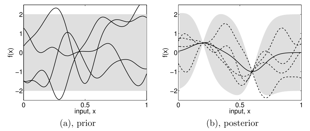
Subfigure (a) shows four samples from a prior distribution. (b) shows the situation after two observations have been made. [Rasmussen2006].

Starting from a prior distribution of functions, it represents the belief we have on the problem. Without any assumption, the mean would be null. If we are now given a dataset \(D = \{(x_1, y_1), (x_2, y_2)\}\), we only consider the function that actually pass through or close to these points, as in the previous figure. This is the learning phase. The more points are added, the more the model will fit the function. Indeed, as we add observations, the error is reduced at these points.

The nature of the covariance matrix is of great importance as it fixes the properties of the functions to consider for inference. This matrix is also called kernel. Many covariance functions exist and they can be combined to fit specific needs. A common choice is the squared exponential covariance kernel:

\[k(x, x') = \sqrt{\pi}l \sigma_p^2 \exp{- \frac{(x - x')^2}{2(\sqrt{2}l)^2}},\]

with \(l\) the length scale, an hyperparameter, which depends on the magnitudes of the parameters. When dealing with a multidimensional case and non-homogeneous parameters, it is of prime importance to adimentionize everything as one input could bias the optimization of the hyperparameters.

Then the Gaussian process regression is written as a linear regression

\[\begin{split}\hat{f}(x_*)&= \sum_{i = 1}^{n}\alpha_i k (x_i, x_*),\\ \alpha &= (K + \sigma_n^2 I)^{-1}y.\end{split}\]

One of the main benefit of this method, is that it provides an information about the variance

\[\mathbb{V}[f(\mathbf{x}_*)] = k(\mathbf{x}_*, \mathbf{x}_*)-\mathbf{k}(\mathbf{x}_*)^T(K + \sigma_n^2 I)^{-1}\mathbf{k}(\mathbf{x}_*).\]

The Kriging method is one of the most employed as of today. We can even enhance the result of the regression if we have access to the derivative (or even the hessian) of the function [Forrester2009]. This could be even more challenging if we don’t have an adjoint solver to compute it. Another method is to use a multi-fidelity metamodel in order to obtain an even better solution. This can be performed if we have two codes that compute the same thing or if we have two grids to run from.

3.3. Polynomial chaos expansion

Some citations: [Blatman2009phd] [Lemaitreknio2010] [Migliorati2013] [Sudret2008] [Xiu2010] [Xiu2002]

Polynomial chaos expansion (PCE) is a type of surrogate model widely used in uncertainty quantification studies. It takes place in a stochastic framework where model inputs are random variables whose probabilistic distributions determine the families of polynomial regressors. We set out below the details of a PCE construction and its implementation with BATMAN.

3.3.1. Generalities

3.3.1.1. Input scaling

Let \(\mathbf{X}=(X_1, X_2, \ldots, X_d)\) be the random input vector defined in the input physical space \(\mathbb{X}\subset\mathbb{R}^d\). The \(i^{\text{th}}\) component \(X_i\) of \(\mathbf{X}\) is transformed into a new random variable \(\zeta_i\) obtained by the following centering and scaling operation:

\[\tilde{X}_i:=\frac{X_i-\mu_i}{\sigma_i}\]

where \(\mu_i=N^{-1}\sum_{k=1}^Nx_i^{(k)}\) and \(\sigma_i=\sqrt{(N-1)^{-1}\sum_{k=1}^N\left(x_i^{(k)}-\mu_i\right)^2}\) are respectively the empirical mean and standard deviation of \(X_i\) computed from a \(N\)-sample \((\mathbf{X}^{(1)},\mathbf{X}^{(2)},\ldots,\mathbf{X}^{(N)})\). The random vector \(\tilde{X}=(\tilde{X}_1,\tilde{X}_1,\ldots,\tilde{X}_d)\) evolves in a space noted \(\tilde{\mathbb{X}}\).

3.3.1.2. Polynomial expansion

Let \(\mathbf{Y}=(Y_1,Y_2,\ldots,Y_p)=f(\mathbf{X})\) be the random model output with values in \(\mathbb{R}^p\). Assuming that the model output \(Y_j\) is of finite variance, each component \(Y_j\) can be considered as a random variable for which there exists a polynomial expansion of the form:

\[Y_j = \displaystyle\sum_{i > 0}\,\gamma_{j,i}\,\Psi_{i}\left(\tilde{\mathbf{X}}\right)=:y_j(\mathbf{X}).\]

where \(\lbrace\Psi_{i}\rbrace_{i\geq 0}\) is a basis of orthonormal polynomial functions:

\[<\Psi_i, \Psi_j> = \delta_{ij}\]

with \(<f, g>\equiv\int_{\tilde{\mathbb{X}}} f(\tilde{\mathbf{x}})g(\tilde{\mathbf{x}}) \rho(\tilde{\mathbf{x}}) \mathrm{d}\tilde{\mathbf{x}}\) and \(\delta_{ij}\) the Kronecker delta function,

and where \(\gamma_{j,i}\) is the coefficient of the projection of \(y_j\) onto \(\Psi_i\):

\[\gamma_{j,i}=<y_j, \Psi_i>.\]

3.3.1.3. Polynomial basis

In practice, this orthonormal basis is built using the tensor product of \(d\) 1-D polynomial functions coming from \(d\) different orthonormal basis:

\[\Psi_i(\tilde{\mathbf{x}})=\Psi_{i_1(i)}(\tilde{x}_1)\otimes\Psi_{i_2(i)}(\tilde{x}_2)\otimes\ldots\otimes\Psi_{i_d(i)}(\tilde{x}_d),\]

where \(\left(i_1(i),i_2(i),\ldots,i_d(i)\right)\in\mathbb{N}^d\) is the multi-index associated to the integer \(i\in\mathbb{N}\). The bijective application \(i_{1,2,\ldots,d}=(i_1,i_2,\ldots,i_d):\mathbb{N}\rightarrow\mathbb{N}^d\) is an enumerate function to chose (see Enumerate strategies).

The choice for the basis functions depends on the probability measure of the random input variables \(\zeta_1,\zeta_2,\ldots,\zeta_d\). According to the Askey’s scheme, the Hermite polynomials form the optimal basis for random variables following the standard Gaussian distribution:

\[\forall n\in\mathbb{N},~H_{n+1}(x) = xH_n(x) - nH_{n-1}(x) \text{ with }H_{0}(x)=1\text{ and }H_{1}(x)=x\]

and the Legendre polynomials are the counterpart for the standard uniform distribution:

\[\forall n\in\mathbb{N},~L_{n+1}(x) = \frac{2n+1}{n+1}xL_n(x) - \frac{n}{n+1}L_{n-1}(x) \text{ with }L_{0}(x)=1\text{ and }L_{1}(x)=x.\]

Note that even if standard uniform and Gaussian distributions are widely used to represent input variable uncertainty, the Askey’s scheme can also be applied to a wider set of distributions [Xiu2002].

3.3.1.4. Surrogate model

From a deterministic point of view, for a given realization \(\mathbf{x}\) of \(\mathbf{X}\) and based on the previous variable change, we have:

\[y_j\left(\mathbf{x}\right):=\displaystyle\sum_{i \geq 0}\,\gamma_{j,i}\,\Psi_{i}\left(\tilde{\mathbf{x}}\right).\]

In practice, we use a truncation strategy (see Truncation strategies) limiting this polynomial expansion to the more significant elements in terms of explained output variance:

\[\hat{y}_j\left(\mathbf{x}\right):=\displaystyle\sum_{i = 0}^r\,\gamma_{j,i}\,\Psi_{i}\left(\tilde{\mathbf{x}}\right).\]

Thus, \(\hat{\mathbf{y}}=(\hat{y}_1,\hat{y}_2,\ldots,\hat{y}_p)\) is a surrogate model of \(\mathbf{y}=(y_1,y_2,\ldots,y_p)\).

3.3.2. Properties

Various statistical moments associated to the PC surrogate model have explicit formulations, thus avoiding Monte-Carlo sampling, even if this metamodel is computationally cheap.

For the \(j^{\text{th}}\) output, the expectation reads:

\[\mathbb{E}\left[\hat{y}_j\left(\mathbf{X}\right)\right]=\gamma_{j,0}\]

For the \(j^{\text{th}}\) output, the variance reads:

\[\mathbb{V}\left[\hat{y}_j\left(\mathbf{X}\right)\right]=\sum_{i = 1}^r\gamma_{j,i}^2\]

For the \(j^{\text{th}}\) and \(k^{\text{th}}\) outputs, the expectation reads:

\[\mathbb{C}\left[\hat{y}_j,\hat{y}_k\left(\mathbf{X}\right)\right]=\sum_{i = 1}^r\gamma_{j,i}\gamma_{k,i}\]

In the context of global sensitivity analysis, there are similar results for the Sobol’ indices [Sudret2008].

3.3.3. Options

3.3.3.1. Enumerate strategies

Remind that:

• \(\forall i\in\{0,1,\ldots,r\},~\Psi_i(\tilde{\mathbf{x}})=\Psi_{1,i_1(i)}(\tilde{x}_1)\otimes\Psi_{2,i_2(i)}(\tilde{x}_2)\otimes\Psi_{d,i_d(i)}(\tilde{x}_d)\).

• \(\forall k\in\{1,2,\ldots,d\},~\{\Psi_{k,i}\}_{0\leq i \leq P}\) are the \(P+1\) first elements of the polynomial basis associated to \(X_k\) and their degrees are lower or equal to \(P\).

• \(\forall i\in\{0,1,\ldots,r\},~\forall k\in\{1,2,\ldots,d\},~\text{degree}(\Psi_{k,i_k(i)})=i_k(i)\leq P\).

• \(\forall i\in\{0,1,\ldots,r\},~\text{degree}(\Psi_{i})=\sum_{k=1}^d\text{degree}(\Psi_{k,i_k(i)})\leq P\).

An enumerate function is a bijective application from \(\{0,1,\ldots,P\}\) to \(\{0,1,\ldots,P\}^d\) of the form:

\[i\mapsto i_{1,2,\ldots,d}(i)=(i_1(i),i_2(i),\ldots,i_d(i)).\]

The bijectivity property implies that the initial term is:

\[i_{1,2,\ldots,d}(0)=\{0,0,\ldots,0\}\]

and the next ones satisfy the constraint:

\[\forall 0\leq i \leq j,~ \text{degree}(\Psi_i)<\text{degree}(\Psi_j) \Leftrightarrow \forall 0\leq i \leq j,~ \sum_{k=1}^d i_k(i) < \sum_{k=1}^d i_k(j)\]

or

\[\forall 1\leq i \leq j,~\exists m \in\{1,2,\ldots,d\}:~(\forall k\leq m,~i_k(i)=i_k(j))~\text{ and }~ (i_m(i)<i_m(j)).\]

Linear enumerate function

A natural linear enumerate strategy is the lexicographical order with a constraint of increasing total degree. The unique requirement of this strategy is the input space dimension \(d\).

Hyperbolic anisotropic enumerate function

Hyperbolic truncation strategy gives an advantage to the main effects and low-order interactions. From a multi-index point of view, this selection implies to discard multi-indices including an important number of non-zeros components.

\(\forall q \in ]0, 1]\), the anisotropic hyperbolic norm of a multi-index \(\boldsymbol{\alpha}\in\mathbb{R}^d\) is defined by:

\[\| \boldsymbol{\alpha} \|_{\mathbf{w}, q} = \left( \sum_{k=1}^{d} w_k \alpha_k^q \right)^{1/q}\]

where the \(w_k\)‘s are real positive numbers. In the case where \(\mathbf{w}=(1,1,\ldots,1)\), the strategy is isotropic.

3.3.3.2. Truncation strategies

In this section, we present different truncation strategies.

Note that for small \(d\), advanced truncation strategies that consist in eliminating high-order interaction terms or using sparse structure [Blatman2009phd] [Migliorati2013] are not necessary.

Fixed truncation strategy

The standard truncation strategy consists in constraining the number of terms \(r\) by the number of random variables \(d\) and by the total polynomial degree \(P\) of the PCE. Precisely, the choice of \(r\) is equal to:

\[r = \frac{(d + P)!}{d!\,P!}.\]

All the polynomials \(\Psi_i\) involving the \(d\) random variables with a total degree less or equal to \(P\) are retained in the PC expansion. Then, the PC approximation of \(y_j\) is formulated as:

\[\widehat{y}_j(\mathbf{x}) = \displaystyle\sum_{0\leq i \leq r}\,\gamma_{j,i}\,\Psi_i\left(\tilde{\mathbf{x}}\right) = \displaystyle\sum_{i\in\mathbb{N}\atop\sum_{k=1}^di_k(i)\leq P}\,\gamma_{j,i}\,\Psi_i\left(\tilde{\mathbf{x}}\right).\]

Warning

The number of terms \(r\) grows polynomially both in \(d\) and \(P\) though, which may lead to difficulties in terms of computational efficiency and memory requirements when dealing with high-dimensional problems.

Sequential truncation strategy

The sequential strategy consists in constructing the basis of the truncated PC iteratively. Precisely, one begins with the first term \(\Psi_0\), that is \(K_0 = \{0\}\), and one complements the current basis as follows: \(K_{i+1} = K_i \cup \{\Psi_{i+1}\}\). The construction process is stopped when a given accuracy criterion is reached, or when \(i\) is equal to a prescribed maximum basis size \(r\).

Cleaning truncation strategy

The cleaning strategy aims at building a PC expansion containing at most \(r\) significant coefficients, i.e. at most \(r\) significant basis functions. It proceeds as follows:

• Generate an initial PC basis made of the \(r\) first polynomials (according to the adopted EnumerateFunction), or equivalently an initial set of indices \(\mathcal{I} = \{0, \ldots, r-1\}\).

• Discard from the basis all those polynomials \(\Psi_i\) associated with insignificance coefficients, i.e. the coefficients that satisfy:

\[|\gamma_i| \leq \epsilon \times \max_{ i' \in \mathcal{I} } |\gamma_{i'}|\]

where \(\epsilon\) is the significance factor, default is \(\epsilon = 10^{-4}\).

• Add the next basis term \(\Psi_{i+1}\) to the current basis \(\mathcal{I}\).

• Reiterate the procedure until either \(r\) terms have been retained or if the given maximum index \(r_{\text{max}}\) has been reached.

3.3.3.3. Coefficient calculation strategies

We focus here on non-intrusive approaches to numerically compute the coefficients \(\lbrace\gamma_{j,i}\rbrace_{0\leq i \leq r\\ 1\leq j \leq p}\) using \(N\) snapshots from \(\mathcal{D}_N\).

Least-square strategy

Based on a \(N\)-sample \(\left(\mathbf{X}^{(k)},\mathbf{Y}^{(k)}\right)_{1\leq k \leq N}\), the least-square strategy seeks the solution of the optimization problem:

\[\hat{\boldsymbol{\gamma}}=\underset{\boldsymbol{\gamma}\in\mathbb{R}^r}{\operatorname{argmin}} \sum_{k=1}^N \sum_{j=1}^p \left(y_j^{(k)}-\displaystyle\sum_{0\leq i \leq r}\,\gamma_{j,i}\,\Psi_i\left(\tilde{\mathbf{x}}^{(k)}\right)\right)^2\]

which is achieved through classical linear algebra tools.

Note that the sample size \(N\) required by this strategy is at least equal to \(p(r+1)\) where \(r\) is the number of PC coefficients and \(p\) is the output vector dimension.

Quadrature strategy

The spectral projection relies on the orthonormality property of the polynomial basis. For the \(j^{\text{th}}\), the \(i^{\text{th}}\) coefficient \(\gamma_{j,i}\) is computed using a Gaussian quadrature rule as:

\[\gamma_{j,i} = <y_j,\Psi_i> \,\cong\,\displaystyle\sum_{k = 1}^{N}\,y_j^{(k)}\,\Psi_i(\tilde{\mathbf{x}}^{(k)})\,w^{(k)}\]

where:

• \(\mathbf{y}^{(k)} = \mathcal{M}(\mathbf{x}^{(k)})\) is the evaluation of the simulator at the \(k^{\text{th}}\) quadrature root \(\tilde{\mathbf{x}}^{(k)}\) of \(\Psi_i\),

• \(w^{k}\) is the weight associated to \(\mathbf{x}^{(k)}\).

Note that the number of quadrature roots required in each uncertain direction to ensure an accurate calculation of the integral \(<y_j,\Psi_i>\) is equal to \((P+1)\).

3.3.4. Implementation

Concerning the library BATMAN, polynomial chaos expansion has to be specified in the block surrogate of the JSON settings file, setting the keyword method at pc and eventually using ones of the following keywords:

Keywords	Type	Description
strategy	string	Strategy for the weight computation: least square: LS quadrature: Quad
degree	integer	Total polynomial degree \(P\)
distributions	list(openturns.Distribution)	Distributions of each input parameter
n_sample	integer	Number of samples for least square

3.4. Multifidelity

It is possible to combine several level of fidelity in order to lower the computational cost of the surrogate building process. The fidelity can be either expressed as a mesh difference, a convergence difference, or even a different set of solvers. [Forrester2006] proposed a way of combining these fidelities by building a low fidelity model and correct it using a model of the error:

\[\hat{f}(x) = f_c(x) + \hat{f}_{\epsilon}(f_e(x), f_c(x)),\]

with \(\hat{f}_{\epsilon}\) the surrogate model representing the error between the two fidelity levels. This method needs nested design of experiments for the error model to be computed.

Considering two levels of fidelity \(f_e\) and \(f_c\), respectively an expensive and a cheap function expressed as a computational cost. A cost ratio \(\alpha\) between the two can be defined as:

\[\alpha = \frac{f_e}{f_c}.\]

Using this cost relationship an setting a computational budget \(C\), it is possible to get a relation between the number of cheap and expensive realizations:

\[\begin{split}C f_e &= N_e f_e + N_c f_c,\\ C f_e &= N_e f_e + N_c\frac{\alpha}{f_e},\\ C &= N_e + N_c\alpha, \\ N_c &= \frac{C - N_e}{\alpha}.\end{split}\]

As the design being nested, the number of cheap experiments must be strictly superior to the number or expensive ones. Indeed, the opposite would result in no additional information to the system.

3.5. Mixture of expert

The prediction based on surrogate models can be false when a bifurcation occurs. In such case a solution is found with the Local Decomposition Method (LDM) [Dupuis2018]. It seeks to find separate the input parameter space into sub-spaces depending on the physics. These sub-spaces are called clusters and are constructed using unsupervised machine learning techniques. Then, local surrogate models are computed on each sub-spaces. In order to predict a new sample points, a classifier constructed using supervised machine learning is used to determine to which cluster it belongs. The sample is then predicted using the right local surrogate model.

Following is the LDM’s algorithm:

1. Computation of PCA on data of higher dimensions than scalars. PCA helps the clusterer to find patterns in the data.

2. Clustering using unsupervised machine learning.

3. Formation of local surrogate models.

4. Classification using supervised machine learning.

5. Prediction of new points using the local models according to their cluster affiliations.

3.5.1. Clustering using Unsupervised Machine Learning

Unsupervised machine learning tools from Scikit-Learn are used to cluster data set according to parameters chosen by the user, especially the number of clusters (clustering documentation). The objective of these methods is to put a label on each data according to their affiliation to a cluster. To cover the majority of possible data types, different methods are used. Among most used methods: KMeans is a distance based method which proposes a fast computation time and simple algorithm; GaussianMixture uses a probabilistic approach (KDE); and DBSCAN is a density-based algorithm.

3.5.2. Predictions using Supervised Machine Learning

The label of each cluster and their data can be used to form local surrogate models for each of these clusters (supervised learning). The construction of each local surrogate model is based on classical methods previously detailed can be used.

To predict new samples, supervised machine learning tools from Scikit-Learn are used to affiliate each point to their clusters then use the corresponding local model to make a prediction. These classifiers use the previously clusterised data set along with the labels (from unsupervised machine learning) to classify new data points called training set by applying what they learnt with the previously clusterised data set called trained set. Again, there are numerous options depending on the nature of the data. Support Vector Classification is used as the default method.

3.6. Example with RAE2822

3.6.1. Step 1: CFD Runs

In this example, the code elsA co-developed at ONERA and CERFACS is used to run CFD simulations on a wing profile. The geometry used for this case is the RAE2822 wing profile from the AS28G aircraft configuration:

This test case is a basic wing profile used to study the interactions between boundary layers and shocks. These interactions can lead to the detachment of the boundary layer which imply lift loss. To control the detachment, we want the shock to be as far as possible on the wing to limit its influence on the pressure around the profile.

Various inflow conditions are simulated in order to characterize the steady flow around the profile. Then, the DoE consists in a set of incidence angle of the inflow and a Mach number.

These CFD runs being expensive, the construction of a surrogate model is required to do such analysis. However, these changes in inflow conditions can lead to the presence of a shock or not on the profile. This causes different regimes which are not governed by the same equations, a bifurcation. Thus, the LDM can be used.

3.6.2. Step 2: Application of Local Decomposition Method

To help seperate our data into clusters, a physical-based sensor that can detects shocks can be used. In this case, the Jameson Shock sensor is used. It can detects discontinuities and nonlinearities:

\[\nu_i = \frac{\mid P_{i+1}-2P_i + P_{i-1}\mid}{\epsilon + \mid P_{i+1}\mid + 2\mid P_i\mid + \mid P_{i-1}\mid},\]

with \(P_i\) the pressure along the wing and \(\epsilon\) a constant to avoid ill posed problems. The sensor is computed for all samples. Its dimension is reduced by PCA to ease the clustering step. KMeans (unsupervised machine-learning) is used to separate the different regimes in the reduced space. In the end each set of input parameters is associated to a given cluster depending on the physics. The position of the clusters in the DoE can be visualized:

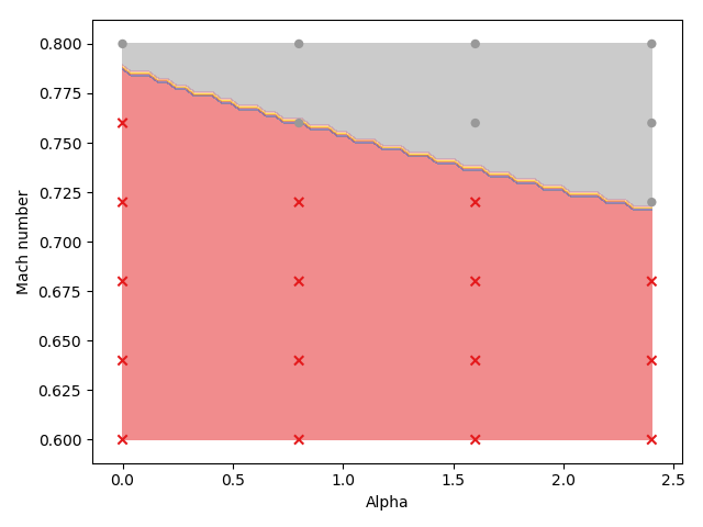
These 2 clusters are used to form 2 local surrogate models by Gaussian Process. The quality of these models is assessed by LOOCV. While a global model gives a quality of \(Q_2=0.60\), the LDM is able to acheave \(Q_2=0.84\). Indeed, the global model tried to model the bifurcation which lead to an overal drop of the quality.

In order to predict new samples, Support Vector Machine (supervised machine-learning) is used to classify these new samples to a given cluster. Based on these associations, the corresponding local models are used to predict the samples.