Mascaret software for hydraulic modelling¶

This section presents the use of BATMAN for uncertainty quantification in the case of hydraulic modelling. Firstly, scientific notions relative to this domain are introduced. Then, different simple test cases are described through the setting files associated with a dedicated software and the UQ treatment is prescribed in the BATMAN setting file. BATMAN is also used for a real study case based on the Garonne river with a consistent part associated with visualization. Lastly, an API developed for this software in order to lead UQ study is presented.

Note

The following test cases require the installation of the MASCARET software and the corresponding API which are not included in the BATMAN library. Visit the website http://www.opentelemac.org to get them.

1. The hydraulic model¶

Free surface flow dynamics in rivers are well modeled by the Navier-Stokes equations (NSE). When the vertical dimension is supposed to be significantly smaller than the horizontal dimensions and when the bathymetry variations are supposed to be small, the shallow-water equations (SWE) can be derived from the NSE, by means of their vertical integration under the hydrostatic pressure assumption. The SWE form a hyperbolic system of partial differential equations, which represents sub-critical and supercritical flows with hydraulic jumps. In the present work, only sub-critical flows of rivers in plains are considered, consistently with the hydraulic model used at operational level for the Garonne river.

One-dimensional models are widely used in hydraulic engineering, for instance in flood forecasting. One-dimensional SWE are derived from two prime principles: mass conservation and momentum conservation. For most applications in rivers, the equations are written in terms of discharge (or flow rate) $Q$ $[\text{m}^3.\text{s}^{-1}]$ and hydraulic section $A$ $[\text{m}^2]$ that relates to water level (or water height) $h$ $[\text{m}]$ such that $A \equiv A(h)$ . The curvilinear abscissa in the simulation domain is denoted by $s$ ranging from $s_\text{in}$ upstream of the river to $s_\text{out}$ downstream. Thus, the non-conservative form of the one-dimensional SWE reads:

$\Biggl \lbrace { \partial_t A(h)+\partial_s Q = 0 \atop \partial_t Q + \partial_s\left(Q(h)^2/A(h)\right)+gA(h)\partial_s h - gA(h)\left(S_0-S_f\right)=0 }$

with $g~[\text{m}.\text{s}^{-2}]$ the gravity, $S_0$ the channel slope and $S_f$ the friction slope. These equations are usually combined with an equation for the friction slope $S_f$ , here described by the Manning-Strickler formula: $S_f=Q^2K_S^{-2}A(h)^{-2}R(h)^{-4/3}$ where $R(h)=A(h)/P(h)$ is the hydraulic radius written as a function of the wet perimeter $P(h)$ and $K_S~[\text{m}^{1/3}.\text{s}^{-1}]$ is the Strickler friction coefficient.

2. Uncertainty quantification for the MASCARET software¶

In the present application, the MASCARET software is used to simulate the one-dimensional SWE, i.e. the water level $h$ and discharge $Q$ over the discrete hydraulic network for $s\in[s_{\text{in}},s_{\text{out}}]$ . This simulator is commonly used for dam-break wave simulation, reservoir flushing and flooding. The hydraulic model requires the following input parameters: bathymetry, upstream and downstream boundary conditions, lateral inflows, roughness coefficients and initial condition for the hydraulic state $(h,Q)$ .

Some references:

A Finite Volume Solver for 1D Shallow-Water Equations Applied to an Actual River, N. Goutal and F. Maurel, Int. J. Numer. Meth. Fluids 2002; 38:1-19
MASCARET: a 1-D Open-Source Software for Flow Hydrodynamic and Water Quality in Open Channel Networks, N. Goutal, J.-M. Lacombe, F. Zaoui and K. El-Kadi-Abderrezzak, River Flow 2012 – Murillo (Ed.), pp. 1169-1174
Website: http://www.opentelemac.org/index.php/presentation?id=138

In practice, even if the input parameters are set at believable values, some uncertainties remain concerning these choices and turn into uncertainty in the simulated hydraulic state. Analyzing this hydraulic state variability through uncertainty quantification, notably in view of the input ones through sensitivity analysis, is of prime importance e.g. in a risk analysis framework or a data assimilation system.

In what follows, we apply the BATMAN library to an academic test case (a rectangular open channel) and a real hydraulic model (a section of the Garonne river).

3. Test cases for a rectangular open channel¶

We consider a simple rectangular open channel with the following features:

length: $5~\text{km}$
space step: $100~\text{m}$
maximal time: $1~\text{h}$
Strickler coefficient: $30.59~\text{m}^{1/3}.\text{s}^{-1}$
upstream flow: $1000~\text{m}^3.\text{s}^{-1}$
downstream height: $12.5~\text{m}$

We design different test cases using the user configuration file config_canal_user_{TestCaseName}.json required by the Mascaret API. The common features are:

"Q_cst": 0.0 in "init_cst": initial flow rate set to $0~\text{m}^3.\text{s}^{-1}$ everywhere;
"Z_cst": 10.0 in "init_cst": initial water level set to $10~\text{m}$ everywhere;
"info_bc": true in "misc": print information concerning the boundary conditions;
"all_outstate": true in "misc": return the water level at each node.

The uncertain parameters are the Strickler coefficient $K_S$ and the upstream flow rate $Q_{\text{up}}$ , and sometimes the bathymetry.

3.1. Test case #1: simple configuration¶

Source: ./tests_cases/Mascaret/INPUTS/examples_config_canal/config_canal_user_simple.json

This test case is simply defined by the common features.

{
    "init_cst": {
        "Q_cst": 0.0,
        "Z_cst": 10.0
    },
    "misc": {
        "info_bc": true,
        "all_outstate": true,
        "index_outstate": 25
    }
}

3.2. Test case #2: change $K_S$ and $Q_{\text{up}}$ ¶

Source: ./tests_cases/Mascaret/INPUTS/examples_config_canal/config_canal_user_KsQ.json

This test case changes the predefined values of $K_S$ and $Q_{\text{up}}$ and is defined as follows:

the Strickler coefficient $K_S$ ("Ks": {}) is set to $25.0~\text{m}^{1/3}.\text{s}^{-1}$ ("value": 25.0) for the zone ("zone": true) index 0 ("ind_zone": 0);
the upstream flow rate $Q_{\text{up}}$ ("Q_BC": {}) is set to $2345~\text{m}^{3}.\text{s}^{-1}$ ("value": 2345.0) for the zone index 0 ("idx: 0).

{
    "init_cst": {
        "Q_cst": 0.0,
        "Z_cst": 10.0
    },
    "Q_BC": {
        "idx": 0,
        "value": 2345.0
    },
    "Ks": {
        "zone": true,
        "value": 25.0,
        "ind_zone": 0
    },
    "misc": {
        "info_bc": true,
        "all_outstate": true
    }
}

3.3. Test case #3: change the bathymetry uniformly¶

Source: ./tests_cases/Mascaret/INPUTS/examples_config_canal/config_canal_user_bathy.json

This test case changes the predefined value of the bathymetry ("bathy": {}) and is defined as follows:

all bathymetry sections are modified ("all_bathy": true);
the increase is set to $2~\text{m}$ ("dz": 2.0) at each section.

{
    "init_cst": {
        "Q_cst": 0.0,
        "Z_cst": 10.0
    },
    "bathy": {
        "all_bathy": true,
        "dz": 2.0
    },
    "misc": {
        "info_bc": true,
        "all_outstate": true
    }
}

3.4. Test case #4: change the bathymetry non-uniformly¶

Source: ./tests_cases/Mascaret/INPUTS/examples_config_canal/config_canal_user_bathyLp.json

This test case changes the predefined value of the bathymetry ("bathy": {}) and is defined as follows:

all bathymetry sections are modified ("all_bathy": true)
the variation is defined by a centered Gaussian process with a squared exponential kernel (use of "Lp");
the correlation length of the Gaussian process is set to $222~\text{m}$ ("Lp": 222.0);
the standard deviation of the Gaussian process is set to $2~\text{m}$ ("dz": 2.0).

{
    "init_cst": {
        "Q_cst": 0.0,
        "Z_cst": 10.0
    },
    "bathy": {
        "all_bathy": true,
        "dz": 2.0,
        "Lp": 222.0
    },
    "misc": {
        "info_bc": true,
        "all_outstate": true
    }
}

3.5. BATMAN setting file for these test cases¶

3.5.a. Input parameter space¶

Test cases #1, #2 and #3

Sources:

./tests_cases/Mascaret/INPUTS/examples_settings_canal/settings_KsQ.json (UQ-Mascaret)
./tests_cases/Mascaret/INPUTS/examples_settings_canal/settings_kriging_KsQ.json (UQ-Kriging)
./tests_cases/Mascaret/INPUTS/examples_settings_canal/settings_PC_KsQ.json (UQ-PCE)

We define the input parameters:

$K_{S_3}\in[20.0, 40.0]$ ,
$Q_{\text{up}}\in[1000.0, 3000.0]$ .

We suppose that:

$K_{S_3}$ follows an uniform distribution over $[20.0, 40.0]$ ,
$Q_{\text{up}}$ follows a Beta distribution over $[20.0, 40.0]$ with mean set to 2000 and standard deviation set to 500.

"space": {
    "corners": [
        [20.0, 1000.0],
        [40.0, 3000.0]
    ],
    "sampling": {
        "init_size": 120,
        "method": "saltelli",
        "distributions": [
            "Uniform(20., 40.)",
            "BetaMuSigma(2000, 500, 1000, 3000).getDistribution()"
        ]
    }
}

Test case #4

Source: ./tests_cases/Mascaret/INPUTS/examples_settings_canal/settings_bathy.json

We only consider the bathymetry as input parameter. We do not specify a probability distribution for the bathymetry because by definition, the bathymetry is a Gaussian process defined by the configuration file config_canal_user_bathyLp.json. We want to make 5 snapshots using a Halton sequence.

"space": {
    "corners": [
        [999.0, 999.0],
        [9999.0, 9999.0]
    ],
    "sampling": {
        "init_size": 5,
        "method": "halton"
    }
}

3.5.b. Snapshot provider¶

We configure the snapshot provider itself. We specify that no more than 5 can be simultaneous run. We define the name of the header and output file as well as the dimension of the output. Here BATMAN will look at the variable "F", which is a vector of size 51, within the file function.dat. It corresponds to the values of the input parameter "x1" and "x2" stored in the file "header.py". The BASH script file of the provider is "script.sh" and is situated in the directory "data". The input values are stored in the directory "batman-data" and the input-output snapshots are stored in the directory "cfd-output-data".

"snapshot": {
    "max_workers": 5,
    "plabels": ["x1", "x2"],
    "flabels": ["X", "F"],
    "io": {
        "point_filename": "point.json",
        "data_filename": "point.dat",
        "data_format": "fmt_tp_fortran"
    },
    "provider": {
        "type": "file",
        "context_directory": "data",
        "coupling_directory": "batman-coupling",
        "command": "bash script.sh",
        "clean": false
    }
}

The BASH script file of the provider calls the Python file function.py.

#!/bin/sh

python function.py > function.out

The Python file function.py creates an instance of the class MascaretApi which depends of the configuration test case file (here 'config_garonne_lnhe.json') and configuration user file ('config_garonne_lnhe_user.json'). Then, it reads the input parameter values stored in './batman-data/header.py' and makes a conversion to floating format. The Mascaret software is run with these input parameter values using the function __call__ of the class MascaretApi. The water level F is printed and plotted. Lastly, the input-output snapshot is stored in ./cfd-output-data/function.dat.

#!/usr/bin/env python
# coding:utf-8

import re
import json
import numpy as np
import ctypes
import csv
from batman.input_output import (IOFormatSelector, Dataset)
from batman.functions import MascaretApi

study = MascaretApi('config_garonne_lnhe.json','config_garonne_lnhe_user.json')

# Input from header.py
with open('./batman-coupling/point.json', 'r') as fd:
    params = json.load(fd)

X1 = params['x1']
X2 = params['x2']

X1 = float(X1)
X2 = float(X2)

# Function
X, F = study(x=[X1, X2])

# Output
nb_value = np.size(X)
with open('./batman-coupling/point.dat', 'w') as f:
    f.writelines('TITLE = \"FUNCTION\" \n')
    f.writelines('VARIABLES = \"X\" \"F\"  \n')
    f.writelines('ZONE T=\"zone1\" , I=' + str(nb_value) + ', F=BLOCK  \n')
    for i in range(len(X)):
        f.writelines("{:.7E}".format(float(X[i])) + "\t ")
        if i % 1000:
            f.writelines('\n')
    f.writelines('\n')

    for i in range(len(F)):
        f.writelines("{:.7E}".format(float(F[i])) + "\t ")
        if i % 1000:
            f.writelines('\n')
        f.writelines('\n')

3.5.c. Data visualization¶

The design of experiments is not plotted ("doe": false). 5 ticks are used on the colorbar. The cost function is labeled "F(Ks, Q)". The curvilinear abscissa associated with the output components are stored in "xdata" (from 0 to 5 km with interval set to 100 m). This optionnal block provides a response surface of the water level "F" in function of the input parameter "Ks" and "Q".

"visualization": {
    "doe": false,
    "xdata": [0.0, 100.0, 200.0, 300.0, 400.0, 500.0, 600.0, 700.0, 800.0, 900.0, 1000.0, 1100.0, 1200.0, 1300.0, 1400.0, 1500.0, 1600.0, 1700.0, 1800.0, 1900.0, 2000.0, 2100.0, 2200.0, 2300.0, 2400.0, 2500.0, 2600.0, 2700.0, 2800.0, 2900.0, 3000.0, 3100.0, 3200.0, 3300.0, 3400.0, 3500.0, 3600.0, 3700.0, 3800.0, 3900.0, 4000.0, 4100.0, 4200.0, 4300.0, 4400.0, 4500.0, 4600.0, 4700.0, 4800.0, 4900.0, 5000.0],
    "ticks_nbr": 5,
    "flabel": "F(Ks, Q)"
}

3.5.d. Uncertainty quantification¶

We compute the "aggregated" "Sobol" indices based on a sample of size 1200 with the distributions:

uniform distribution over $[20.0, 40.0]$ for $K_{S_3}$ ,
Beta distribution over $[20.0, 40.0]$ with mean set to 2000 and standard deviation set to 500 for $Q_{\text{up}}$ .

"uq": {
    "sample": 1200,
    "pdf": [
        "Uniform(20., 40.)",
        "BetaMuSigma(2000, 500, 1000, 3000).getDistribution()"
    ],
    "type": "aggregated",
    "method": "sobol"
}

4. Test case for the Garonne river between Tonneins and La Réole¶

We also consider a real hydraulic network over the Garonne river in France. The Garonne river flows from the Pyrenees to the Atlantic Ocean in the area of Bordeaux. It is approximately $647-\text{km}$ long and drains an area of $55'000~\text{km}^2$ . The present study focuses on a $50-\text{km}$ reach from Tonneins ( $s = 13~\text{km}$ ) to La R’eole ( $s = 62~\text{km}$ ) with an observation station at Marmande ( $s = 36~\text{km}$ ). The mean slope over the reach is $S_0=3.3~\text{m}.\text{km}^{-1}$ and the mean width of the river is $W=250~\text{m}$ . The bank-full discharge is approximately equal to the mean annual discharge ( $Q_0=1'000~\text{m}^3.s^{-1}$ ). Despite the existence of active floodplains, this reach can be modeled accurately by a 1-D hydraulic model.

The hydraulic model for the the Garonne River is built from 83 on-site bathymetry cross sections from which the full 1D bathymetry is interpolated. Friction is prescribed over 3 portions for the river channel and the floodplain; it is represented by the Strickler coefficients $K_{S_1},K_{S_2},K_{S_3}$ . It should be noted that Marmande is located at the beginning of the $K_{S_3}$ portion. The upstream boundary condition is prescribed with an unsteady flow $Q_{\text{up}}(t)$ ; the downstream boundary condition is prescribed with a local rating curve established at La R’eole that sets $h(s_{\text{out}})=h_{\text{out}}$ . The hydraulic model has been calibrated using channel and floodplain roughness coefficients as free parameters.

4.1. Description of the test case¶

Source: ./tests_cases/Mascaret/INPUTS/examples_config_garonne/config_garonne_lnhe_user_KsQ.json

This test case changes the predefined values of $K_{S_3}$ and $Q_{\text{up}}$ and is defined as follows:

the Strickler coefficient $K_S$ ("Ks": {}) is set to $32.0~\text{m}^{1/3}.\text{s}^{-1}$ ("value": 32.0) for the zone ("zone": true) index 2 ("ind_zone": 2);
the upstream flow rate $Q_{\text{up}}$ ("Q_BC": {}) is set to $2345~\text{m}^{3}.\text{s}^{-1}$ ("value": 2345.0) for the zone index 0 ("idx: 0).

We print information concerning the boundary conditions ("info_bc": true) and consider the water level at each space step ("all_outstate": true).

{
    "Q_BC": {
        "idx": 0,
        "value": 2345.0
    },
    "Ks": {
        "zone": true,
        "value": 32.0,
        "ind_zone": 2
    },
    "misc": {
        "info_bc": true,
        "all_outstate": true
    }
}

4.2. Parametrizing the BATMAN settings file for a UQ study¶

We can also realize a UQ study using the JSON settings file. For the Garonne test case, the sources of uncertainty are $Q$ and $K_{S_3}$ and their probabilistic distributions are described from expert knowledge. Both Strickler coefficient $K_{S_3}$ and bank-full discharge $Q_{\text{up}}$ follow uniform distributions and are supposed to be independent:

	$K_{S_3}$	$Q_{\text{up}}$
Distribution	Uniform( $\text{min},\text{max}$ )	Normal( $\text{mean},\text{std}$ )
Parameter #1	$\text{min}=15$	$\text{mean}=4031$
Parameter #2	$\text{max}=60$	$\text{std}=400$

Goal:

Build a design of experiments
Build a surrogate model from this design of experiments
Evaluate the Sobol’ indices associated to the variables $Q_{\text{up}}$ and $K_{S_3}$

Source: ./tests_cases/Mascaret/INPUTS/examples_settings_garonne/settings_PC_KsQ_gauss.json

To run these tasks, go to the directory ./test_cases/Mascaret/. and use the commande line:

./install_links_run_mascaret_garonne_lnhe
cp INPUTS/examples_settings_garonne/settings_PC_KsQ_gauss.json .
batman settings_PC_KsQ_gauss.json -uq

where:

settings_PC_KsQ_gauss.json is the path of the settings file,
u is the option for carrying out an uncertainty quantification study,
q is the option for estimating Q2 and finding the point with max MSE.

4.2.1. Design of experiments¶

"space": {
    "corners": [
        [15.0, 1000.0],
        [60.0, 6000.0]
    ],
    "sampling": {
        "init_size": 121,
        "method": "halton",
        "distributions": ["Uniform(15., 60.)", "Normal(4031, 400)"]
    }
}

We define a design of experiments where:

the lower bounds of $(K_{S_3},Q_{\text{up}})$ are [15.0, 1000.0],
the upper bounds of $(K_{S_3},Q_{\text{up}})$ are [60.0, 6000.0],
the design method is Halton sequencing,
the sample size is equal to 121,
the distribution of $K_{S_3}$ is "Uniform(15., 60.)",
the distribution of $Q_{\text{up}}$ is "Normal(4031, 400)",

4.2.2. Generation of snapshots¶

We configure the snapshot provider itself. We specify that no more than 5 can be simultaneous run. We define the name of the header and output file as well as the dimension of the output. Here BATMAN will look at the variable "F", which is a vector of size 463, within the file function.dat. It corresponds to the values of the input parameter "x1" and "x2" stored in the file "header.py". The BASH script file of the provider is "script.sh" and is situated in the directory "data". The input values are stored in the directory "batman-data" and the input-output snapshots are stored in the directory "cfd-output-data".

"snapshot": {
    "max_workers": 5,
    "plabels": ["x1", "x2"],
    "flabels": ["X", "F"],
    "io": {
        "point_filename": "point.json",
        "data_filename": "point.dat",
        "data_format": "fmt_tp_fortran"
    },
    "provider": {
        "type": "file",
        "context_directory": "data",
        "coupling_directory": "batman-coupling",
        "command": "bash script.sh",
        "clean": false
    }
}

4.2.3. Surrogate model¶

Based on the snapshot sample obtained from the previous steps (see 4.2.1. Design of experiments and 4.2.2. Generation of snapshots), we define a metamodel with the following features:

the type is a polynomial chaos expansion (PCE): "method": "pc",
the PCE weights are estimated by truncation: "strategy": "Quad",
the total polynomial degree is fixed to 10: "degree": 10.

and make "predictions" for the following $(K_{S_3}, Q_{\text{up}})$ values of [[30, 2000]].

"surrogate": {
    "predictions": [[30, 2000]],
    "method": "pc",
    "strategy": "Quad",
    "degree": 10
},

4.2.4. Uncertainty quantification¶

In the UQ study, we use the PCE metamodel instead of the Mascaret simulator which is too CPU-time expensive. Based on the computational technique called "aggregated", we estimate the "Sobol"’ indices associated with the Strickler coefficient $K_{S_3}$ whose distribution is "Uniform(15., 60.)" and the flow rate $Q_{\text{up}}$ whose distribution is "Normal(4031, 400)" using a sample whose size is equal to 50000.

"uq": {
    "sample": 50000,
    "pdf": ["Uniform(15., 60.)", "Normal(4031, 400)" ],
    "type": "aggregated",
    "method": "sobol"
}

4.2.5. Visualization¶

The design of experiments is not plotted ("doe": false). 5 ticks are used on the colorbar. The cost function is labeled "F(Ks, Q)". The curvilinear abscissa associated with the output components are stored in "xdata" (from 13.150 km to 62.175 km). This optionnal block provides a response surface of the water level "F" in function of the input parameter "Ks" and "Q".

"visualization": {
    "doe": false,
    "xdata": [13150.0, 13250.0, 13350.0, ..., 62056.25, 62175.0],
    "ticks_nbr": 5,
    "flabel": "F(Ks, Q)"
}

4.3. Examples of figures¶

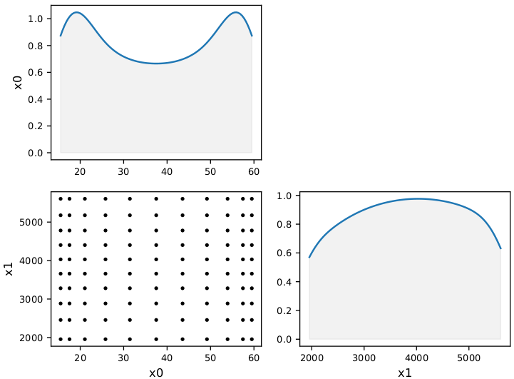
Design of experiments:

Plot of the design of experiments with the empirical distribution ( $x_0$ corresponds to the input parameter $K_{S_3}$ and $x_1$ corresponds to the input parameter $Q$ ).

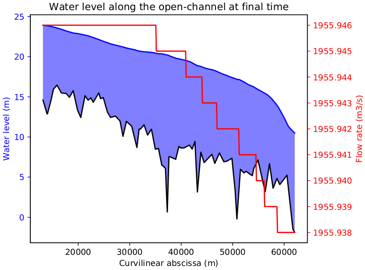
Water level for the first snapshot

Plot of the water level (blue line) and flow rate (red line) at final simulation time along the open-channel. The bathymetry is plotted in dark.

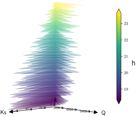
3D Kiviat plot

Representing the 120-sample by means of a 3D Kiviat where the output is represented by a surface whose colour corresponds to the value and extremities corresponds to the input values.

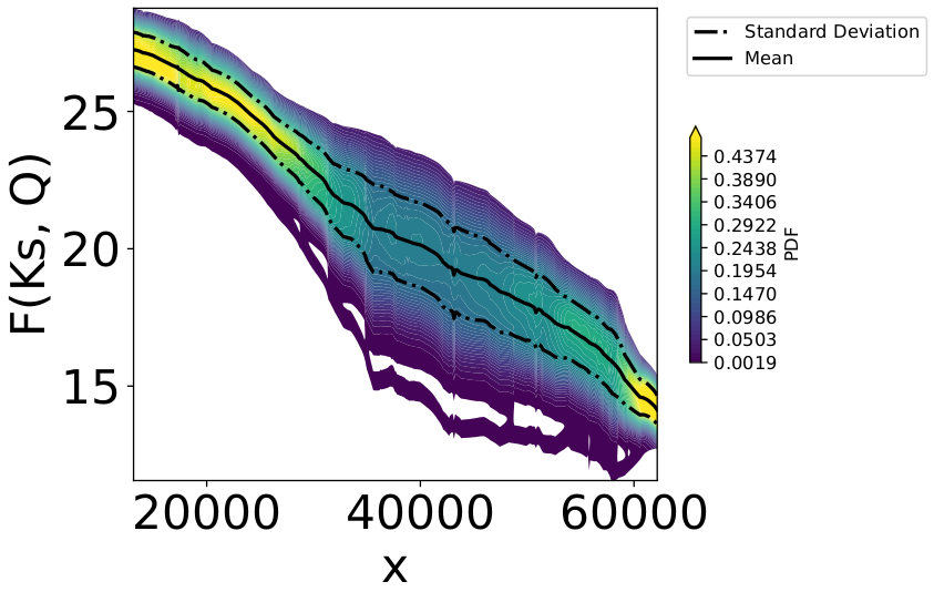
Output probability density function

Plot of the probability density function of the water level evaluated at each spatial point.

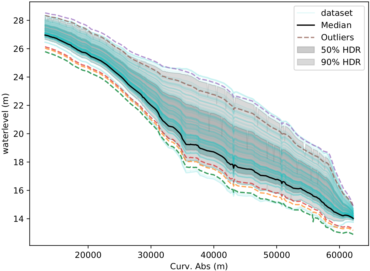
Highest density region plot

Plot of the highest density region plot of the water level where the black line represents the median, both gray areas represent the 50% and 90% confidence intervals and the dashed lines represent the outliers present in the dataset.

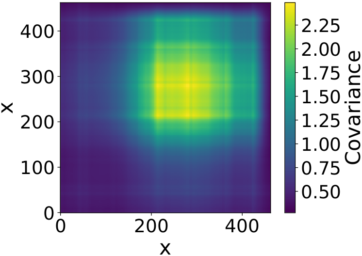
Output covariance plot

Plot of the covariance of the water level at the different spatial points.

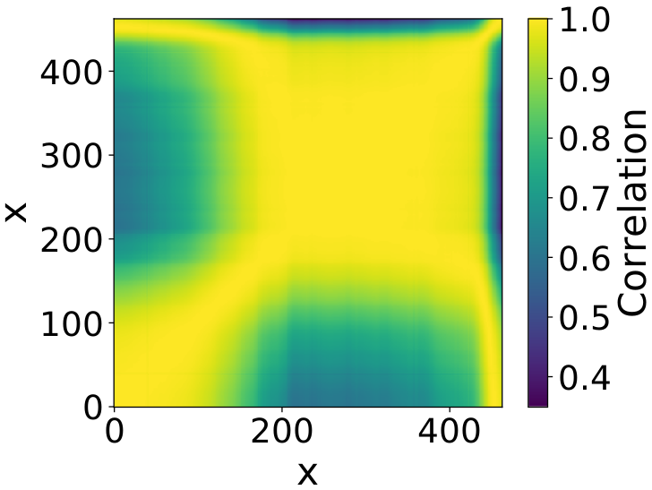
Output correlation plot

Plot of the correlation of the water level at the different spatial points.

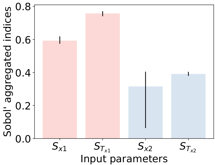
Aggregated Sobol’ indices

Plot of the Sobol’ indices associated to the input parameters $K_{S_3}$ (here denoted $x_1$ ) and $Q$ (here denoted $x_2$ ), with a confidence interval symbolized by a black segment.

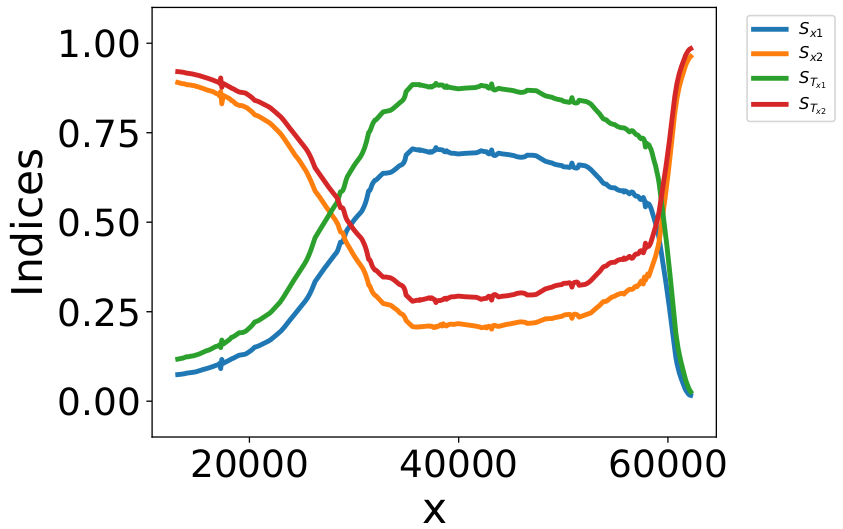
Regionalized Sobol’ indices

Plot of regionalized the Sobol’ indices associated to the input parameters $K_{S_3}$ (here denoted $x_1$ ) and $Q$ (here denoted $x_2$ ). We can see that these sensitivity change along the river.

5. Use of the Mascaret API¶

Source: ./tests_cases/Mascaret/test_run.py

5.1. Import packages and functions¶

import ctypes
import csv
import numpy as np
import os
from collections import OrderedDict
from batman.functions import MascaretApi
from batman.functions.telemac_mascaret import print_statistics, histogram, plot_opt

5.2. Read the MascaretApi documentation¶

# Details about MascaretApi
help(MascaretApi)

5.3. List the different test cases¶

# Create the dictionary of model and user config files
files = OrderedDict()
# -- CANAL
files["canal", "model"] = 'config_canal.json'
files["canal", "user"] = 'config_canal_user.json'
files["canal", "install"] = './install_links_run_mascaret_canal'
# -- GARONNE_LNHE
files["garonne_lnhe", "model"] = 'config_garonne_lnhe.json'
files["garonne_lnhe", "user"] = 'config_garonne_lnhe_user.json'
files["garonne_lnhe", "install"] = './install_links_run_mascaret_garonne_lnhe'
# -- GARONNE_LNHE_CASIER
files["garonne_lnhe_casier", "model"] = 'config_garonne_lnhe_casier.json'
files["garonne_lnhe_casier", "user"] = 'config_garonne_lnhe_casier_casier.json'
files["garonne_lnhe_casier", "install"] = './install_links_run_mascaret_garonne_lnhe_casier'
# -- ADOUR
files["adour", "model"] = 'config_adour.json'
files["adour", "user"] = 'config_adour_user.json'
files["adour", "install"] = './install_links_run_mascaret_adour'

5.4. Select and install the test case environment¶

# Let the user to select one of these test cases
i = 0
for i in range(len(files) / 3):
    print('- Test case #{}: {}'.format(i+1, files.keys()[i*3][0]))
id_test_case = input('Select one of these test cases (index)... ')
test_case = files.keys()[(int(id_test_case)-1)*3][0]
print('- Your selected test case: {}'.format(test_case))

# Install the environment corresponding to this test case
os.system(files[test_case, "install"])

5.5. Build the corresponding Mascaret model and print information¶

# Create an instance of MascaretApi
study = MascaretApi(files[test_case, "model"], files[test_case, "user"])

# Print informations concerning the study specified in the JSON file
print(study)

5.6. Run the Mascaret model with values specified in command line¶

# Run study with Ks and Q specified constant values
print('RUNNING MASCARET WITH SPECIFIED VALUES OF KS AND Q')
Ks = float(input('Specify the value (e.g. 30) of KS = '))
Q = float(input('Specify the value (e.g. 3000) of Q = '))
h = study(x=[Ks, Q])
if len(h)==1:
    print('The water level computed with Ks = {} and Q = {} is {}.'.format(Ks, Q, h[0]))
else:
    for i, _ in enumerate(h):
        print('The water level #{} computed with Ks = {} and Q = {} is {}.'.format(i, Ks, Q, h[i]))
plot_opt('ResultatsOpthyca.opt')

5.7. Run the Mascaret model with values specified in the user settings file¶

# Run study with the user defined tasks and values
print('RUNNING MASCARET WITH JSON USER DEFINED VALUES OF KS AND Q')
h = study()
if len(h)==1:
    print('The water level computed with json user defined values is {}.'.format(h[0]))
else:
    for i, _ in enumerate(h):
        print('The water level #{} computed with json user defined values is {}.'.format(i, h[i]))
plot_opt('ResultatsOpthyca.opt')