Michalewicz function
Introduction
Examples can be found in BATMAN’s installer subrepository test-cases. To create a new study, use the same structure as this example on the Michalewicz function:
Michalewicz
|
|__ data
|   |__ script.sh
|   |__ function.py
|
|__ settings.json
The working directory consists in two parts:
data: contains all the simulation files necessary to perform a new simulation. It can be a simple python script to a complex code. The content of this directory will be copied for each snapshot. In all cases,script.shlaunches the simulation.settings.json: contains the case setup.
Note
The following section is a step-by-step tutorial that can be applied to any case.
Michalewicz Function
Step 1: Simulation directory
For this tutorial, the Michalewicz function was choosen. It is a multimodal d-dimensional function which has  local minima - for this test-case:

where m defines the steepness of the valleys and ridges.
Note
- It is to difficult to search a global minimum when
 reaches large value. Therefore, it is recommended to have
  .
. - In this case we used the two-dimensional form, i.e.
 .
.
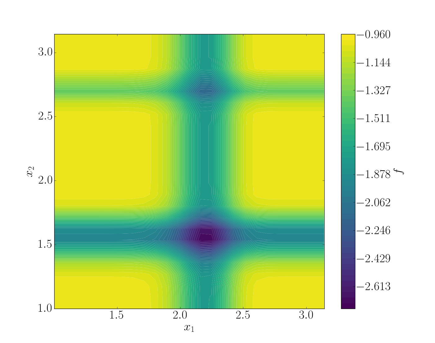
To summarize, we have the Michalewicz 2*D* function as follows:

See also
For other optimization functions, read more at this website.
- Create the case for BATMAN
For each snapshot, BATMAN will copy the content of data and add a new folder batman-coupling which contains a single file point.json. The content of this file is updated per snapshot and it only contains the input parameters to change for the current simulation. Hence, to use Michalewicz’s function with BATMAN, we need to have this file read to gather input parameters.
Aside from the simulation code and this headers, there is a script.sh. It is this script that is launched by BATMAN. Once it is completed, the computation is considered as finished. Thus, this script manages a solver launch, calls a python script, etc.
In the end, the quantity of interest has to be written in tecplot format within the directory batman-coupling.
Note
These directories’ name and path are fully configurables.
Note
For a simple function script, you can pass it directly in the settings file.
Step 2: Setting up the case
BATMAN’s settings are managed via a python file located in scripts. An example template can be found within all examples directory. This file consists in five blocks with different functions:
- Block 1 - Space of Parameters
The space of parameters is created using the two extrem points of the domain here we have ![x_1, x_2 \in [1, \pi]^2](../_images/math/dab184734370993fe08a82f7b791c272373ac52b.svg) . Also we want to make 50 snapshots using a halton sequence.
. Also we want to make 50 snapshots using a halton sequence.
"space": {
    "corners": [
        [1.0, 1.0],
        [3.1415, 3.1415]
    ],
    "sampling": {
        "init_size": 50,
        "method": "halton"
    },
}
- Block 2 - Snapshot provider
Then, we configure the snapshot itself. We define the name of the header and output file as well as the dimension of the output. Here BATMAN will look at the variable F, which is a scalar value, within the file point.dat.
"snapshot": {
    "max_workers": 10,
    "parameters": ["x1", "x2"],
    "variables": ["F"],
    "provider": {
        "type": "file"
        "command": "bash script.sh",
        "context_directory": "data",
        "coupling_directory": "batman-coupling",
        "clean": false
    },
    "io": {
        "point_filename": "point.json",
        "data_filename": "point.dat",
        "data_format": "fmt_tp_fortran"
    }
}
Note
For a simple python function, you can pass it directly in the settings file:
"provider": {
    "type": "plugin",
    "module": "python_module",
    "function": "func_name"
}
with module the name of the python module containing the function function. For an example, see test_cases/Ishigami.
- Block 3 - POD
In this example, a POD is not necessary as it will result in only one mode. However, its use is presented. We can control the quality of the POD, chose a re-sampling strategy, etc.
"pod": {
    "dim_max": 100,
    "quality": 0.8,
    "tolerance": 0.99,
    "type": "static"
}
- Block 4 - Surrogate
A model is build on the snapshot matrix to approximate a new snapshot. The Kriging method is selected. To construct a response surface, we need to make predictions.
surrogate = {'method' : 'kriging',
             'predictions' : [[1., 2.], [2., 2.]],
             }
To fill in easily predictions, use the script prediction.py.
Block 5 - UQ
Once the model has been created, it can be used to perform a statistical analysis. Here, Sobol’ indices are computed using Sobol’s method using 50000 samples.
"uq": {
    "sample": 50000,
    "pdf": ["Uniform(1., 3.1415)", "Uniform(1., 3.1415)"],
    "type": "aggregated",
    "method": "sobol"
}
Step 3: Running BATMAN
To launch BATMAN, simply call it with:
batman settings.json -qsu
BATMAN’s log are found within BATMAN.log. Here is an extract:
BATMAN main ::
    POD summary:
    modes filtering tolerance    : 0.99
    dimension of parameter space : 2
    number of snapshots          : 50
    number of data per snapshot  : 1
    maximum number of modes      : 100
    number of modes              : 1
    modes                        : [ 2.69091785]
batman.pod.pod ::
    pod quality = 0.45977, max error location = (3.0263943749999997, 1.5448927777777777)

----- Sobol' indices -----
batman.uq ::
    Second order: [array([[ 0.        ,  0.06490131],
       [ 0.06490131,  0.        ]])]
batman.uq ::
    First order: [array([ 0.43424729,  0.49512012])]
batman.uq ::
    Total: [array([ 0.51371718,  0.56966205])]
In this example, the quality of the model is estimated around  which means that the model is able to represents around 46% of the variability of the quantity of interest. Also, from Sobol’ indices, both parameters appears to be as important.
Post-treatment
Result files are separated in 4 directories under output:
Case
|
|__ data
|
|__ settings.json
|
|__ output
    |
    |__ surrogate
    |
    |__ predictions
    |
    |__ snapshots
    |
    |__ uq
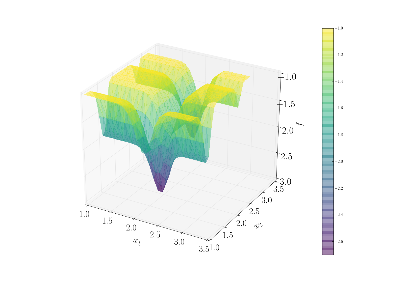
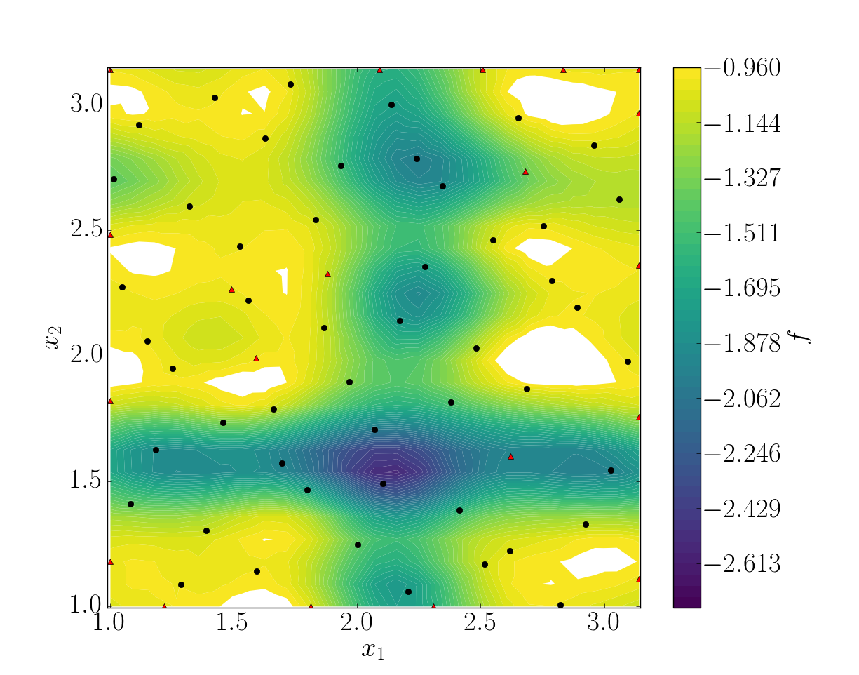
snapshots contains all snapshots computations, predictions contains all predictions, surrogate contains the model and uq contains the statistical analysis. Using predictions we can plot the response surface of the function as calculated using the model:
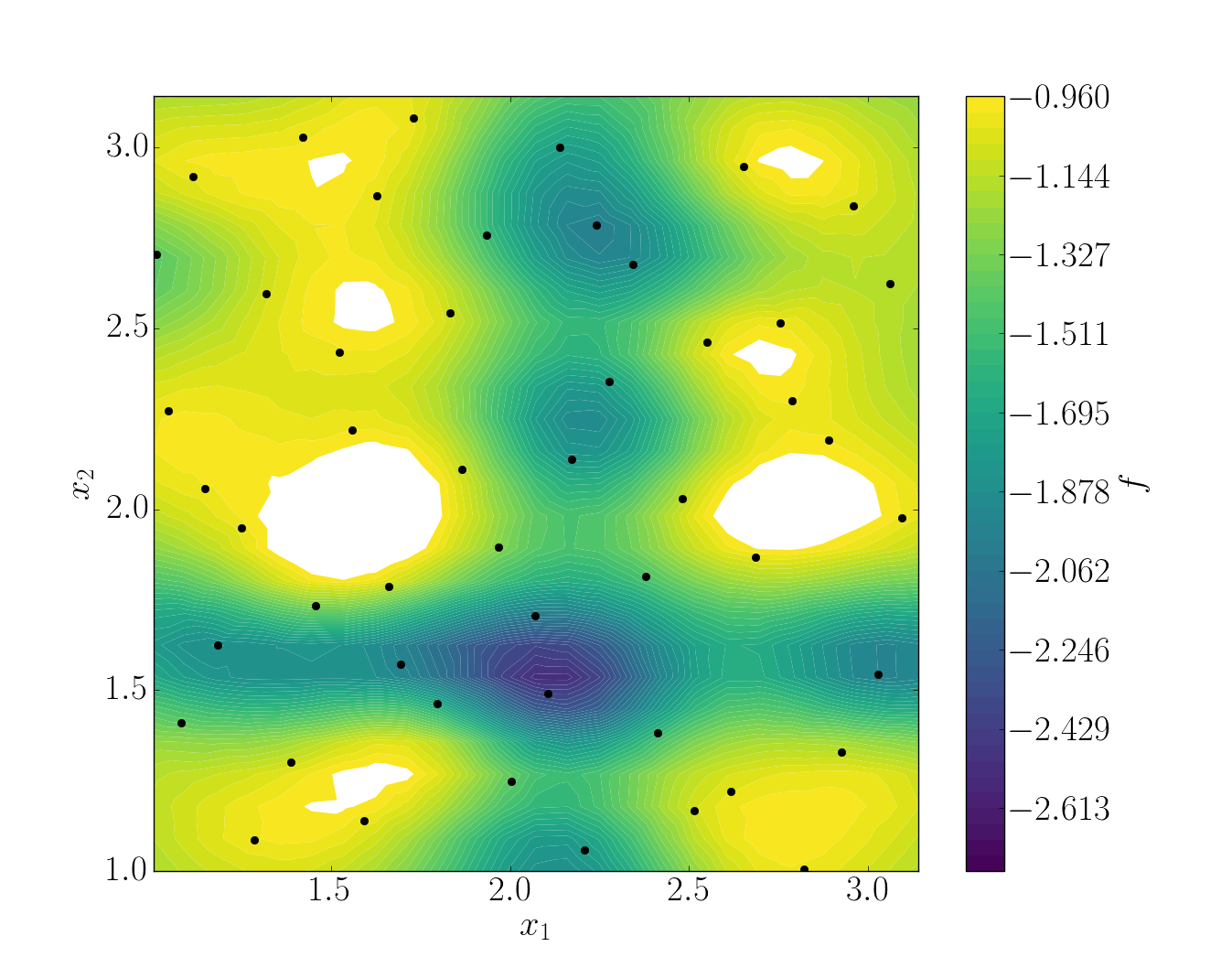
It can be noted that using 50 snapshots on this case is not enought to capture all the non-linearities of the function.
Note
Usually, physical phenomena are smoother. Thus, less points are needed for a 2 parameters problem when dealing with real physics.
Refinement strategies
In this case, the error was fairly high using 50 snapshots. A computation with 50 snapshots using 20 refinement points have been tried. To use this functionnality, the resampling dictionary has to be added:
"resampling":{
        "delta_space": 0.08,
        "resamp_size": 20,
        "method": "loo_sigma",
        "q2_criteria": 0.8
    }
This block tells BATMAN to compute a maximum of 20 resampling snapshots in case the quality has not reach 0.8. This loo_sigma strategy uses the information of the model error provided by the gaussian process regression. This leads to an improvement in the error with  .
.
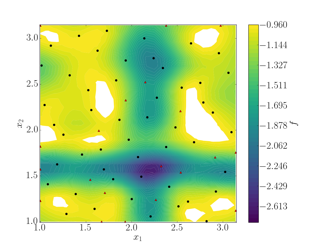
Response surface interpolation using 50 snapshots and 20 refined points, represented by the red triangles.
Using a basic sigma technique with again 20 new snapshots, the error is  .
.
In this case, loo_sigma method performed better but this is highly case dependent.